Highlighting the highest and lowest values with Conditional Formatting

As we mentioned in the introduction, conditional formatting can be used to achieve much more than simply outlining a single entry in a long list. The example in this video shows you how to highlight the cell containing the highest or lowest value respectively.

Drawing attention to highest or lowest value in a list can help you determine priorities. It might be the lowest cost on the list of cars you are looking to buy, or the highest rated associate you are looking to hire. No matter what you choose to use it for, the dynamic nature of conditional formatting allows you to track ranking changes as soon as you input new data.

As you can see in the options menu in the accompanying video, it doesn’t even need to be only one top performer, you can choose to highlight the best 2, 3, 10 (or how many you want) highest or lowest results. This way you can track a wide range of relevant information easily and efficiently.

Highlighting the highest value - step by step:

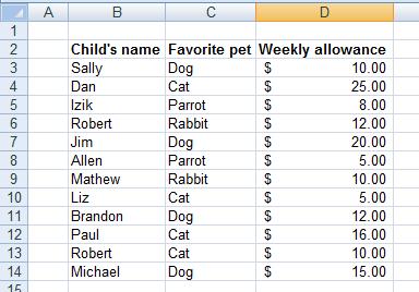
On the following example table, let’s highlight the highest weekly allowance with green color:

1. Start by selecting the relevant range.

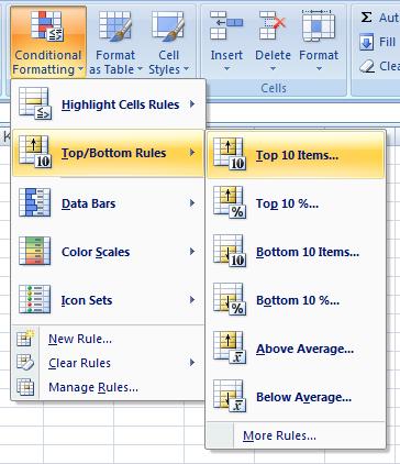
2. Click the “Conditional Formatting” button, and choose “Top/Bottom Rules”, then choose “Top 10 Items”.

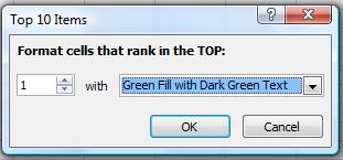
3. Change the “10” into “1” (because we want only the one highest value to be highlighted), and choose the green color.

4. Click OK.

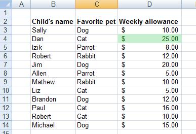
5. Done! you can see the highest value (25) is highlighted with green: